Step-by-step tutorial
This tutorial introduces the foundations of the QMENTA SDK and the technological ecosystem that surrounds it, including Docker and the QMENTA Platform. Its main objective is to guide you through the complete lifecycle of a QMENTA tool: from local implementation and testing, to deployment and execution within the QMENTA Platform.
In QMENTA, a tool is a self-contained piece of software packaged as a Docker image that performs a well-defined computational task on medical data. Tools define their expected inputs, outputs, and execution logic, and can be run reproducibly at scale through the QMENTA Platform. By the end of this tutorial, you will understand how tools are structured, how they interact with the QMENTA Platform, and how to validate that they work correctly before making them available to end users or applying them in large projects.
The final result of this tutorial, including the complete implementation, can be found in this GitHub repository.
As a practical example, we will adapt the ANTs Tutorial, originally implemented as a Python notebook, into a QMENTA tool. The example will use a pair of T1-weighted MRI brain slices as input data. The tool provides several configurable input settings, allowing users to select which ANTs processing steps to execute:
Perform bias field correction
Run tissue segmentation
Compute cortical thickness
Register two images using nonlinear registration.
The tissue segmentation step must be executed before cortical thickness estimation, as the latter depends on the segmentation results. For this reason, these two steps are linked within the tool. All other steps are independent and can be run separately.
In addition, the tool provides a dedicated setting that allows users to fine-tune the analysis by adjusting a specific segmentation parameter.
The resulting tool will extract some statistics, segment anatomical neuroimaging data (2D slice) and report the segmentation results in the online viewer, demonstrating how an existing analysis pipeline can be transformed into a reusable and deployable QMENTA tool. In case you are curious, you can check what kind of tools QMENTA has already available in the QMENTA Tools Catalog.

Note
Advanced Normalization Tools (ANTs) is a C++ library available through the command line that computes high-dimensional mappings to capture the statistics of brain structure and function. It allows one to organize, visualize and statistically explore large biomedical image sets. Additionally, it integrates imaging modalities in space + time and works across species or organ systems with minimal customization.
Note
This tutorial uses ANTs, which is installed via Python. If you plan to use other tools such as FreeSurfer, MATLAB, or MRtrix, they must be fully installed on your system. To ensure these tools are available in the testing or deployment environment, you need to include their installation in your Docker image. This involves adding the necessary installation commands and dependencies to the Dockerfile. You can also check if an official Docker image for the software you want to use already exists and use it as base image, this can save you a lot of time and effort.
Before you begin
To complete this tutorial, you will need the following:
Your favorite IDE or text editor.
Basic knowledge of Python and its ecosystem.
A QMENTA Platform account. You can create a new account in this registration page.
Docker installed in your system. Check their getting started guide to know more about that.
A DockerHub account to register your image.
The example data provided here: a T1 of a segmentated brain r16, and a T1 of a segmentated brain r64.
A
python>=3.10environment with theqmenta-sdk-libandantspyx>=0.6.1libraries installed:pip install qmenta-sdk-lib "antspyx>=0.6.1"
Getting your processing tool in the QMENTA Platform involves several well-defined steps that transform a local script into a reusable, executable component of the QMENTA Platform. At a high level, the process includes the following stages:
Implement the tool logic by writing the main Python script that performs the desired computation and handles inputs and outputs according to the tool specification.
Define the execution environment by creating a Docker image that contains all required dependencies, libraries, and system configurations needed for the tool to run reproducibly.
Test the tool locally to ensure that the code and Docker container behave as expected before deployment.
Register and deploy the tool in the QMENTA Platform.
Run the command tool-maker and it should launch the graphical user interface of the Tool Maker.
/home/myfolder$ tool-maker
It will show something similar to the following screenshot:
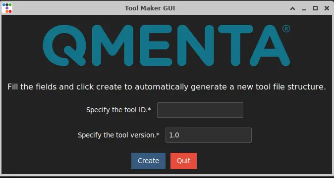
Enter a tool ID (it only accepts lower case letters and “_” character) For example: tool_maker_tutorial. Click on “Create” to create the basic tool file structure.
Generated Files:
/home/myfolder/local_tools/
                   └─ tool_maker_tutorial
                          ├─ description.html
                          ├─ local
                          │    ├─ Dockerfile
                          │    ├─ requirements.txt
                          │    └─ test
                          │        ├─ sample_data
                          │        └─ test_tool.py
                          └─ tool.py
Open you code editor inside the created local_tools/tool_maker_tutorial folder.
Write the main Python program
Input definition and configuration
Open the file tool.py. You can see the basic imports are already created and the class for the tool is written. We are going to use ants as well
so make sure you import it in the top of the file:
import ants
Let’s start editing the method tool_inputs().
These settings define the minimum requirements and configuration options that must be satisfied before the tool can start processing. They describe which input data is required, how that data is selected, and which processing steps will be executed. Together, they form the user-facing interface of the tool in the QMENTA Platform and ensure that the analysis is configured correctly and consistently.
First, an informational message is displayed to the user, providing a brief description of the tool and its purpose.
The input container defines the medical images required by the tool. In this case, the tool expects anatomical brain images with accepted modalities T1 or T2. Two separate input files are required:
One with ‘r16’ included in the file name.
Another with ‘r64’ included in the file name.
Each input is mandatory, and exactly one file must be provided for each condition. The use of file_filter_condition_name allows
the tool to distinguish between these inputs internally and apply different processing logic if needed. In this case, the filters have the
ids c_image1 and c_image2, they are mandatory (set to 1) and they accept only one file (min_files=max_files=1):
# Add the file selection method:
self.add_input_container(
title="ANTsPY Tutorial input files",
info="<h2>ANTsPY Tutorial</h2>Required inputs:<br><b>• Anatomical brain medical image</b>: " \
"2D image to analyze<br> Accepted modalities: 'T1', 'T2'<br> Two files with different filename content: 'r16' and 'r64'", # text in case we want to show which modalities are accepted by the filter.
anchor=1,
batch=1,
container_id="input_images",
mandatory=1,
file_list=[
InputFile(
file_filter_condition_name="c_image1",
filter_file=FilterFile(
modality=[Modality.T1, Modality.T2],
regex=".*r16.*\\.nii\\.gz",
),
mandatory=1,
min_files=1,
max_files=1,
),
InputFile(
file_filter_condition_name="c_image2",
filter_file=FilterFile(
modality=[Modality.T1, Modality.T2],
regex=".*r64.*\\.nii\\.gz",
),
mandatory=1,
min_files=1,
max_files=1,
),
],
)
Visual separators (horizontal lines and headings) are then used to improve readability and structure in the tool configuration interface:
# Displays an horizontal line
self.add_line()
Next, a multiple-choice input allows the user to select which processing steps to execute. These options correspond to the main stages of the ANTs-based tool, such as bias field correction, tissue segmentation, cortical thickness estimation, and image registration. Default selections are provided to guide typical usage while still allowing flexibility:
self.add_input_multiple_choice(
    id_="perform_steps",
    options=[
        ["do_biasfieldcorrection", "Perform Bias Field Correction"],
        ["do_segmentation", "Perform tissue segmentation"],
        ["do_thickness", "Perform cortical thickness"],
        ["do_registration", "ANTs registration interface"],
    ],
    default=["do_biasfieldcorrection", "do_segmentation"],
    title="Which steps do you want to execute?",
)
Finally, a string input parameter is used to configure the MRF (Markov Random Field) parameters required by the segmentation step. This parameter controls the amount of spatial smoothing and the neighborhood radius used during processing. The value is provided as a string to match the ANTs-style parameter format, making it easy to adapt the tool to different image dimensions or analysis requirements:
self.add_input_string(
    id_="mrf",
    default="[0.2, 1x1]",  # antspy tutorial uses 2D iamge
    title="'mrf' parameters as a string, usually \"[smoothingFactor,radius]\" " \
    "where smoothingFactor determines the amount of smoothing and radius determines " \
    "the MRF neighborhood, as an ANTs style neighborhood vector eg \"1x1\" for a 2D image.",
)
Together, these settings ensure that all necessary inputs and parameters are defined before execution, enabling the tool to run reliably and reproducibly on the QMENTA Platform.
In the auto-generated code you can find a useful link to the different inputs’ definition and configuration, helpful if you have not checked it yet to understand better these lines of code.
Replace the content of the tool_inputs() with this:
def tool_inputs(self):
"""
Define the inputs for the tool. This is used to create the settings.json file.
More information on the inputs can be found here:
https://docs.qmenta.com/sdk/guides_docs/settings.html
"""
# Add the file selection method:
self.add_input_container(
title="ANTsPY Tutorial",
info="Required inputs:<br><b>• Anatomical brain medical image</b>: " \
"2D image to analyze<br> Accepted modalities: 'T1', 'T2'<br> Two files with different filename content: 'r16' and 'r64'", # text in case we want to show which modalities are accepted by the filter.
anchor=1,
batch=1,
container_id="input_images",
mandatory=1,
file_list=[
InputFile(
file_filter_condition_name="c_image1",
filter_file=FilterFile(
modality=[Modality.T1, Modality.T2],
regex=".*r16.*\\.nii\\.gz",
),
mandatory=1,
min_files=1,
max_files=1,
),
InputFile(
file_filter_condition_name="c_image2",
filter_file=FilterFile(
modality=[Modality.T1, Modality.T2],
regex=".*r64.*\\.nii\\.gz",
),
mandatory=1,
min_files=1,
max_files=1,
),
],
)
# Displays an horizontal line
self.add_line()
# Displays a header text
self.add_heading("PyANTs tool can perform the following steps:")
self.add_input_multiple_choice(
id_="perform_steps",
options=[
("do_biasfieldcorrection", "Perform Bias Field Correction"),
("do_segmentation", "Perform tissue segmentation"),
("do_thickness", "Perform cortical thickness"),
("do_registration", "ANTs registration interface"),
],
default=[
"do_biasfieldcorrection",
"do_segmentation",
"do_thickness",
"do_registration"
],
title="Which step/s do you want to execute?",
)
# Displays an horizontal line
self.add_line()
self.add_input_string(
id_="mrf",
default="[0.2, 1x1]", # antspy tutorial uses 2D image
title="'mrf' parameters as a string, usually \"[smoothingFactor,radius]\" " \
"where smoothingFactor determines the amount of smoothing and radius determines " \
"the MRF neighborhood, as an ANTs style neighborhood vector eg \"1x1\" for a 2D image.",
)
Processing code (run)
Next, you will begin implementing the run() function, which is the core entry point of the tool execution.
This method is responsible for orchestrating the full data processing pipeline: preparing the execution environment,
retrieving input data, processing the data, and producing the final results.
As a first step, fetch and download the input data associated with the analysis. Input handling is managed through the QMENTA SDK, which provides utilities to automatically retrieve all inputs defined for the tool. By calling:
self.prepare_inputs(context, logger)
the SDK downloads the input files and stores them internally within the self.inputs object, making them readily available for use during processing.
In this tutorial, the tool uses a single input container named input_images. Within this container, the file_filter_condition_name argument is
used to further refine which files are processed by the tool. This mechanism allows the tool to handle specific subsets of
data when multiple files or modalities are present.
After preparing the inputs, you can access the downloaded files using the following pattern:
c_files_handlers_list = self.inputs.input_images.c_files
The resulting variable, c_files_handlers_list, is a list of file handler objects, where each element represents a single input file.
These handlers expose methods and attributes that allow you to interact with the files, such as retrieving their local paths or
associated metadata. A full list of available functionalities can be found in the SDK documentation.
To obtain the local filesystem path of a file—for example, the first file in the list—you can use:
input_data_path = c_files_handlers_list[0].file_path
To monitor the execution flow and facilitate debugging, you should also initialize a logger. Logging allows you to
track the progress of the tool, record key events (such as when data is downloaded or processing starts), and capture
error messages in a structured way. This is particularly important when tools are executed remotely on the QMENTA Platform,
where logs are often the primary mechanism for understanding what happened during execution.
In our particular example, the first part of the run() method looks like this:
# ============================================================
# INITIAL SETUP
# ============================================================

# Initialize logger
logger = logging.getLogger("main")
logger.info("Tool starting")

# Define and create working directory
output_dir = os.path.join(os.environ.get("WORKDIR", "/root"), "OUTPUT")
os.makedirs(output_dir, exist_ok=True)
os.chdir(output_dir)

# this will report in the QMENTA Platform interface the starting of the tool
context.set_progress(value=0, message="Initializing tool execution")

# Download inputs and populate self.inputs
context.set_progress(message="Downloading input data")
self.prepare_inputs(context, logger)

# Retrieve input image paths
fname1_handler = self.inputs.input_images.c_image1[0]
fname1 = fname1_handler.file_path

# Second image only required if Registration is selected to be done.
fname2 = None
if "do_registration" in self.inputs.perform_steps:
    fname2 = self.inputs.input_images.c_image2[0].file_path
More details about containers, file filters and other input settings can be found in Parameters and Input Files.
To keep track of the files generated by the tool and what needs to be reported we initialize two lists:
# Containers to track outputs
generated_files = []
report_items = []
The settings of the tool, that will be used at a later stage to control the execution
of the ANTs library, are accessible from self.inputs followed by the setting id.
At the top of the tool script, before the class definition, you can include an HTML template that will be used to generate the report:
HTML_TEMPLATE = """
<!DOCTYPE html>
<html>
<head>
    <meta charset="UTF-8">
    <title>Image with Caption</title>
</head>
<body>
{body}
</body>
</html>
"""

BODY_TEMPLATE ="""
<h1>{header}</h1>
<h3>{image_caption}</h3>
<img src="{src_image}" alt="{image_description}" style="max-width: 400px;">
"""
Now it’s time for some heavy lifting: you will process the different steps, checking if the step was selected by the user:
# ============================================================
# PROCESSING PHASE
# ============================================================
logger.info("Starting processing phase")
logger.info("Selected steps:\n{}".format("\n".join(self.inputs.perform_steps)))

img = ants.image_read(fname1)

# --- Bias Field Correction ---
if "do_biasfieldcorrection" in self.inputs.perform_steps:
    logger.info("Running N4 bias field correction")
    image_n4 = ants.n4_bias_field_correction(img)
    image_n4.to_filename("n4_processed.nii.gz")

    generated_files.append("n4_processed.nii.gz")
    report_items.append({
        "header": "N4 Bias Field Correction",
        "image": "n4_bias.png",
        "source_image": image_n4,
        "description": "N4 bias field correction result",
    })

# Enforce dependency: segmentation required for thickness
if "do_thickness" in self.inputs.perform_steps and "do_segmentation" not in self.inputs.perform_steps:
    self.inputs.perform_steps.append("do_segmentation")

# --- Tissue Segmentation ---
if "do_segmentation" in self.inputs.perform_steps:
    logger.info("Running tissue segmentation")
    mask = ants.get_mask(img)

    img_seg = ants.atropos(
        a=img,
        m=self.inputs.mrf,
        c='[2,0]',
        i='kmeans[3]',
        x=mask
    )

    img_seg["segmentation"].to_filename("atropos_processed.nii.gz")
    generated_files.append("atropos_processed.nii.gz")

    report_items.append({
        "header": "Tissue Segmentation",
        "image": "segmentation.png",
        "source_image": img_seg["segmentation"],
        "description": "ANTs Atropos tissue segmentation",
    })

    # --- Cortical Thickness ---
    if "do_thickness" in self.inputs.perform_steps:
        logger.info("Running cortical thickness estimation")
        thickimg = ants.kelly_kapowski(
            s=img_seg["segmentation"],
            g=img_seg["probabilityimages"][1],
            w=img_seg["probabilityimages"][2],
            its=45, r=0.5, m=1
        )

        thickimg.to_filename("thickness_processed.nii.gz")
        generated_files.append("thickness_processed.nii.gz")

        report_items.append({
            "header": "Cortical Thickness",
            "image": "thickness.png",
            "overlay": thickimg,
            "base_image": img,
            "description": "Cortical thickness estimation",
        })

# --- Registration ---
if "do_registration" in self.inputs.perform_steps:
    logger.info("Running image registration")
    fixed = ants.image_read(fname1)
    moving = ants.image_read(fname2)

    tx = ants.registration(
        fixed=fixed,
        moving=moving,
        type_of_transform="SyN"
    )

    warped = tx["warpedmovout"]
    warped.to_filename("warped.nii.gz")
    generated_files.append("warped.nii.gz")

    report_items.append({
        "header": "Image Registration",
        "image": "registration.png",
        "overlay": warped,
        "base_image": fixed,
        "description": "ANTs nonlinear registration result",
    })
In this extension of the ANTs tutorial, we will focus on reporting and visualizing the different processing steps performed by the tool. Specifically, the tool will generate 2D slices from the processed data, convert them into PNG images, and include them in a report that can be viewed online within the QMENTA Platform.
To achieve this, the tool will create the PNG files locally, upload them as output artifacts, and generate an HTML report that embeds the images to illustrate the intermediate and final results of the analysis. This report will then be uploaded to the platform, where it can be accessed directly from the analysis interface.
The configuration of the tool outputs will be covered in detail in the next section. For now, the focus is on producing the necessary PNG images, uploading them, and assembling the HTML report that references these images correctly:
# ============================================================
# REPORTING PHASE (ALL PLOTTING + BODY_TEMPLATE)
# ============================================================
logger.info("Generating report content")

body_content = ""

for item in report_items:
    if "overlay" in item:
        item["base_image"].plot(
            overlay=item["overlay"],
            overlay_cmap="jet",
            filename=item["image"]
        )
    else:
        ants.plot(item["source_image"], filename=item["image"])

    generated_files.append(item["image"])

    body_content += BODY_TEMPLATE.format(
        header=item["header"],
        src_image=item["image"],
        image_description=item["description"],
        image_caption=item["description"],
    )

if body_content:
    report_file = "online_report.html"
    with open(report_file, "w") as f:
        f.write(HTML_TEMPLATE.format(body=body_content))

    generated_files.append(report_file)
We are going to upload the generated results into the QMENTA Platform:
# ============================================================
# UPLOADING PHASE
# ============================================================
logger.info("Uploading outputs to QMENTA Platform")

# Upload original input image for reference
context.upload_file(
    source_file_path=fname1,
    destination_path="input_image.nii.gz",
    modality=fname1_handler.get_file_modality(),
    tags=fname1_handler.get_file_tags(),
)

# Upload all generated outputs
for filename in generated_files:
    context.upload_file(filename, filename)

# this will report in the QMENTA Platform interface that the tool has completed
context.set_progress(value=100, message="Processing completed")

logger.info("Tool execution finished successfully")
That is all you need to have the run() method working.
Output definition and configuration
Next, we will optionally adapt the tool_outputs() method to display the results directly in the QMENTA Platform.
This method is executed in the run() method at the end of the file, as it will be detailed later.
Note that not all outputs are always generated, since the user may choose to execute only a subset of the processing steps.
If the QMENTA Platform cannot find the expected files in the output container, the results view will not be displayed.
This step is therefore optional but recommended for a more complete and user-friendly presentation of the tool outputs:
def tool_outputs(self):
    # Main object to create the results configuration object.
    result_conf = ResultsConfiguration()

    # Add the tools to visualize files using the function add_visualization

    # Online 3D volume viewer: visualize DICOM or NIfTI files.
    papaya_1 = PapayaViewer(title="T1 ANTs segmentation and cortical thickness", width="50%", region=Region.center)
    # the first viewer's region is defined as center

    # Add as many layers as you want, they are going to be loaded in the order that you add them.
    papaya_1.add_file(file="input_image.nii.gz", coloring=Coloring.grayscale)  # base iamge, using the file name
    papaya_1.add_file(file="atropos_processed.nii.gz", coloring=Coloring.custom)  # overlay 1, custom coloring shows different colors for different label values.
    papaya_1.add_file(file="thickness_processed.nii.gz", coloring=Coloring.hot_n_cold)  # overlay 2, hot/cold coloring
    # Add the papaya element as a visualization in the results configuration object.
    result_conf.add_visualization(new_element=papaya_1)

    papaya_2 = PapayaViewer(title="T1 ANTs registration", width="50%", region=Region.right)
    # the second viewer's `region` is defined as right. This is required by the Split() element below, which has the property
    # orientation set to `vertical`. If it is set to horizontal, then you can choose between 'Region.top' or 'Region.bottom'.

    # You can use modality or tag of the output file to select the file to be shown in the viewer.
    papaya_2.add_file(file="input_image.nii.gz", coloring=Coloring.grayscale)  # using the file modality
    papaya_2.add_file(file="warped.nii.gz", coloring=Coloring.red)  # using file tag
    result_conf.add_visualization(new_element=papaya_2)

    # To create a split, specify which ones are the objects to be shown in the split
    split_1 = Split(
        orientation=OrientationLayout.vertical, children=[papaya_1, papaya_2], button_label="Images"
    )
    # The button label is defined because this element goes into a Tab element. The tab's "button_label" property
    # is a label that will appear to select between different viewer elements in the platform.

    html_online = HtmlInject(width="100%", region=Region.center, button_label="Report")
    html_online.add_html(file="online_report.html")
    result_conf.add_visualization(new_element=html_online)

    # Remember to add the button_label in the child objects of the tab.
    tab_1 = Tab(children=[split_1, html_online])
    # Call the function generate_results_configuration_file to create the final object that will be saved in the
    # tool path
    result_conf.generate_results_configuration_file(
        build_screen=tab_1, tool_path=self.tool_path, testing_configuration=False
    )
At the end of the file, you will see this lines:
def run(context):
    ToolMakerTutorial().tool_outputs()
    ToolMakerTutorial().run(context)
The class name will depend on the tool id specified in the GUI (in this case ToolMakerTutorial comes from tool_maker_tutorial).
The calling to tool_outputs() is done when running the local test and it will generate the file results_configuration.json.
Depending where you run the tool, the run(context) will be called by the local test or the QMENTA Platform execution system when deployed to run the
python script. You will learn how to test locally in the next section.
Test the tool locally
At this point you can test the Python program locally.
You will need to add the input files in the local_tools/tool_maker_tutorial/local/test/sample_data directory.
And then you will need to change the file local_tools/tool_maker_tutorial/local/test/test_tool.py to adapt it to you
use case. Replace the file’s path, file_filter_condition_name, modality, and tags in the in_args argument of the test_with_args() method:
in_args={
    "test_name": inspect.getframeinfo(inspect.currentframe()).function,  # returns function name
    "sample_data_folder": "sample_data",  # Name of the folder where the test data is stored
    "input_images": {
        "files": [
            # Relative paths to the input data stored in the sample_data folder
            TestFileInput(
                path="data_r16.nii.gz",
                file_filter_condition_name="c_image1",
                modality=Modality.T1,
                mandatory=1
            ),
            TestFileInput(
                path="data_r64.nii.gz",
                file_filter_condition_name="c_image2",
                modality=Modality.T1,
                mandatory=1
            )
        ],
        "mandatory": 1,
    },
    "perform_steps": [
        "do_registration", "do_biasfieldcorrection", "do_thickness"
    ]
},
Once those requirement are fullfilled, run the test using the pytest module from the folder where local_tools/ is found:
pytest local_tools/tool_maker_tutorial/local/test/test_tool.py::TestTool
Tip
The test needs to be run from the folder in order to work, because the path of the tool is automatically added into the PYTHONPATH at runtime
so the test can import the tool’s modules.
In the following section (Package your tool in a Docker image) you will be able to test the tool packaged in a Docker image, an scenario that represents much more faithfully the execution environment in which the tool will be executed when launched through the QMENTA Platform.
Package your tool in a Docker image
You will be using Docker to test your tool in the environment where it is supposed to be run. The Dockerfile can be found here:
local_tools/tool_maker_tutorial/local/Dockerfile.
You will see it’s based on an ubuntu image, but it does not need to be, you can use a lighter base image as long as it supports the code being executed.
Install the python dependencies in the Docker image using the local_tools/tool_maker_tutorial/local/requirements.txt file.
For this example, create the file if it does not exist and paste this content:
antspyx==0.6.1
qmenta-sdk-lib
Now you are ready to run the tool using Docker. There is another test in the same file test_tool.py to execute the tool inside a container.
That same test will create the Docker container for this tool when it is run:
pytest local_tools/tool_maker_tutorial/local/test/test_tool.py::TestToolDocker
If the Docker container has run successfully, the Docker image is ready to be published.
Locate the run docker image in your system. In our case, it should be tool_maker_tutorial:
$ docker images

IMAGE                                              ID            DISK USAGE    CONTENT SIZE   EXTRA
tool_maker_tutorial:1.0                         9e159e20a47e       1.36GB             0B
After having found it, use it to tag it properly with your namespace:
$ docker tag tool_maker_tutorial:1.0 {namespace}/tool_maker_tutorial:1.0
$ docker images

IMAGE                                              ID            DISK USAGE    CONTENT SIZE   EXTRA
{namespace}/tool_maker_tutorial:1.0            9e159e20a47e       1.36GB             0B
Where {namespace} is the name of the Docker namespace, which should coincide with your DockerHub account username, tool_maker_tutorial is the name of the image repository (tool id) and 1.0 is the version tag (tool version).
Once you have validated that the tool completes successfully, the next step is to register the image in DockerHub. To do so, you will have to log in first:
docker login
At this point you will be prompted for your username and password. Once authenticated, you will be able to push the image to the Docker registry:
docker push {namespace}/tool_maker_tutorial:1.0
For more information about working with Docker images see Working with Docker images.
Publish the tool to the QMENTA Platform
You have two options in order to publish your tool in the QMENTA Platform:
Using the
tool-publisheris the easiest way to publish it. This simple interface will ask you the main required fields and submit them to the QMENTA Platform. Follow the instructions in the Publish your tool in the QMENTA Platform using the Tool Publisher.Use the QMENTA Platform interface: Adding manually a tool to the QMENTA Platform.
Run your tool in the QMENTA Platform
After the successful completion of the previous steps, the tool is ready to be run in the QMENTA Platform.
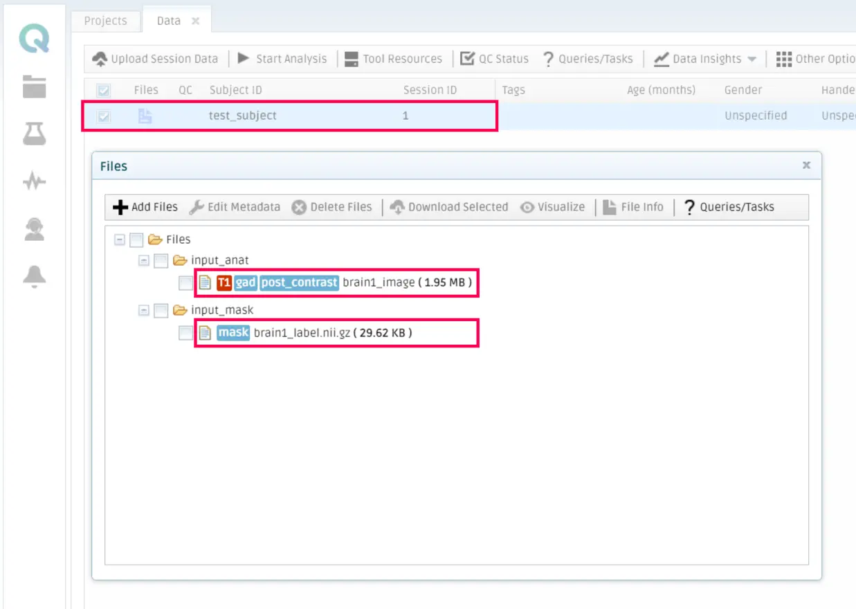
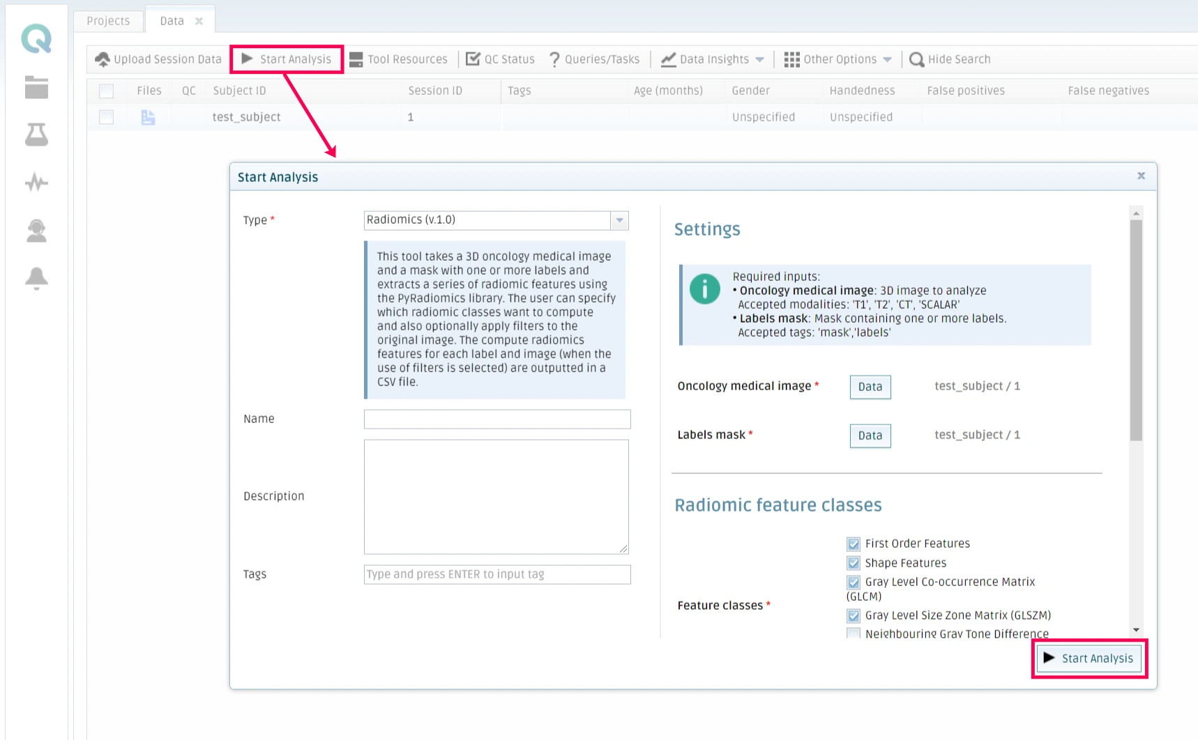
To do so, you should go to My Data in the QMENTA Platform, select a subject that contains the necessary files to run the tool and click on Start Analysis.
Then select your tool, choose the parameters you want it to run with and optionally add a name and a description to the analysis. Click on Start Analysis when the configuration is ready.
The QMENTA Platform will run the analysis and send an email whenever it finishes.
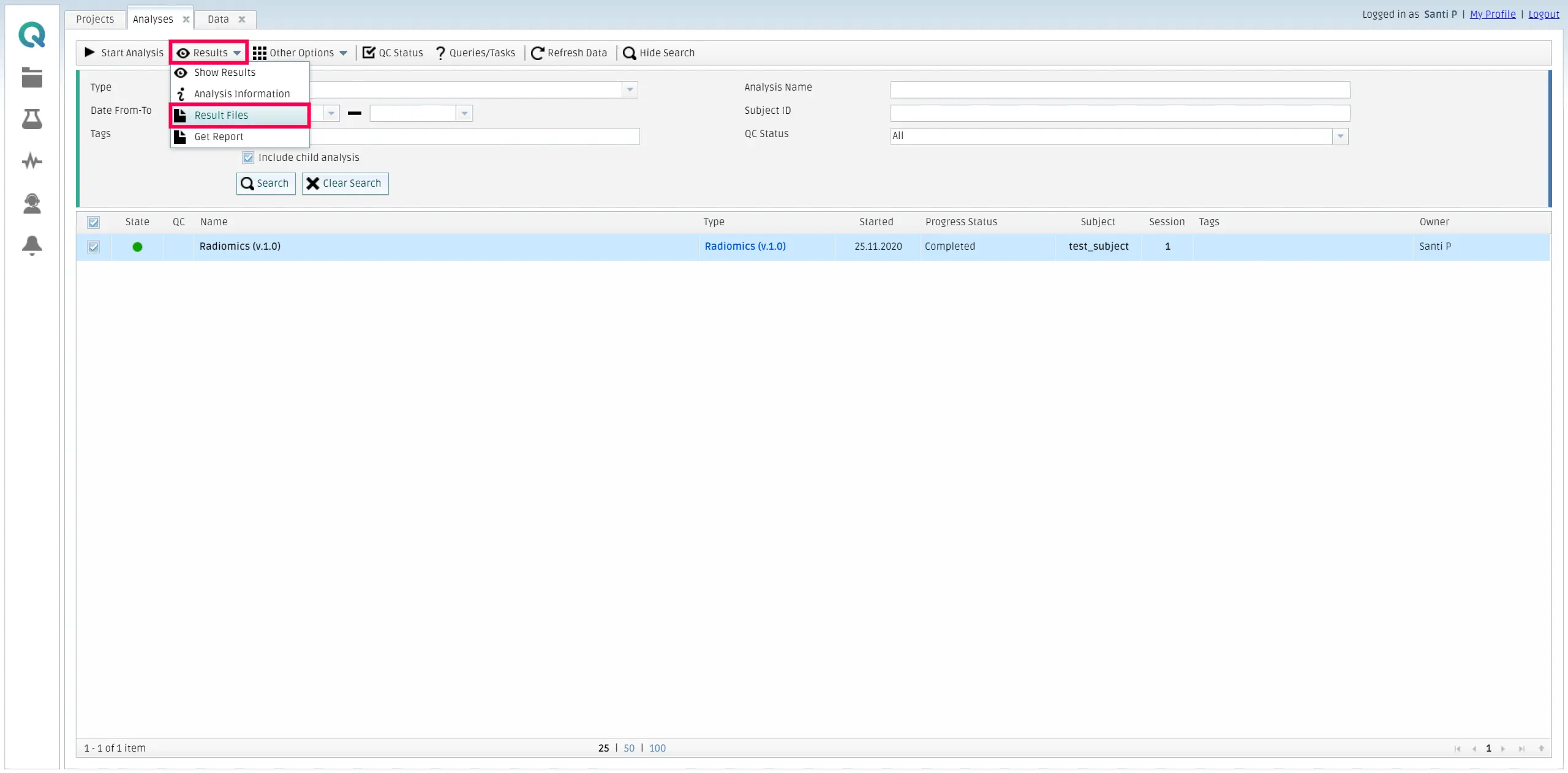
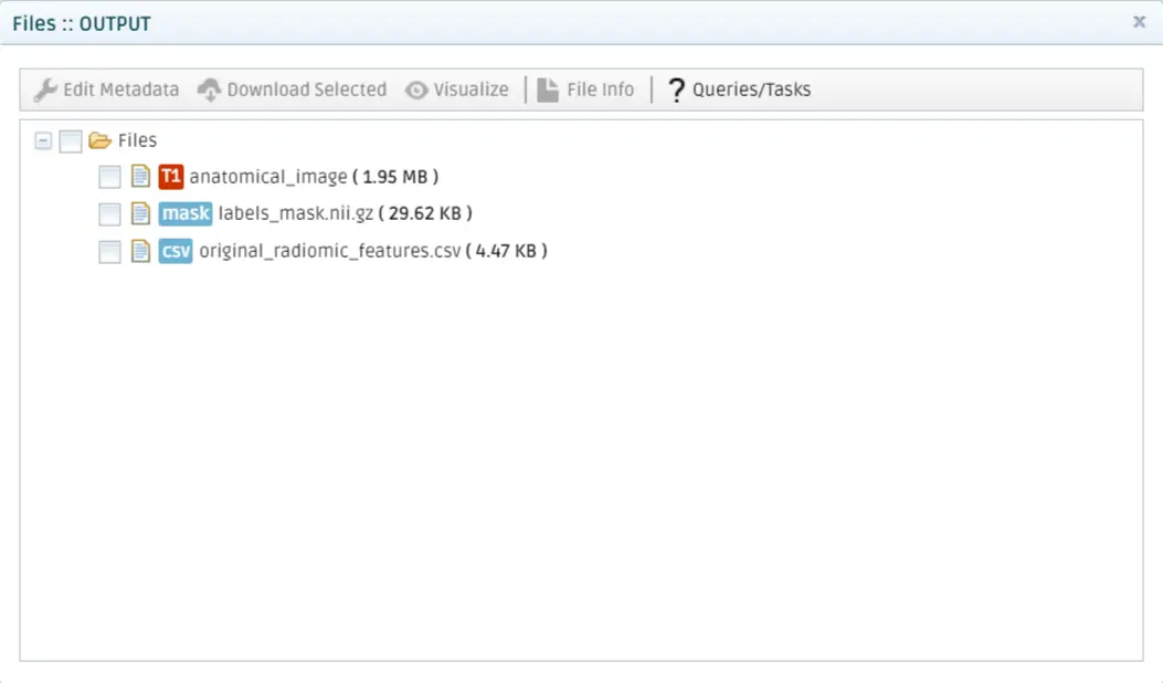
Then, you can retrieve the results by going to My Analysis, selecting the finished analysis, and then click on Results and Result files inside the Results tab.
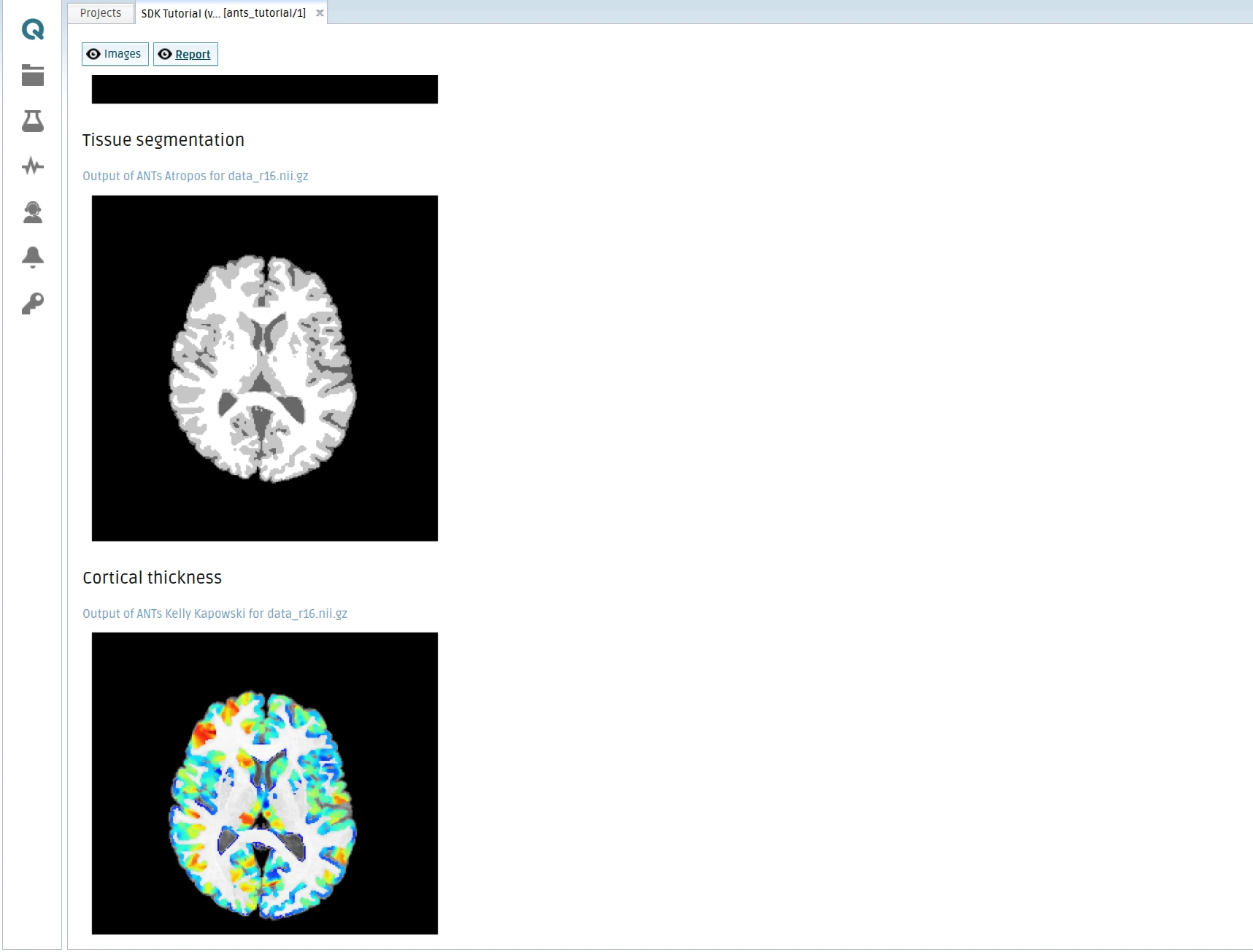
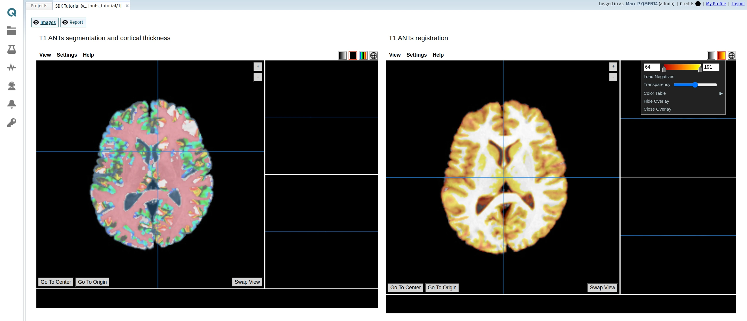
Click on Show Results in the Results dropdown menu to visualize the results. The QMENTA Platform will use the configuration that you set in the Output definition and configuration section of the tool to render the results using the Papaya viewer and display the HTML file set in the configuration to be displayed. Switch views by clicking the buttons on the top left corner.
Papaya viewer with the segmentation and reistration results (Images):
HTML report rendered with the different images showing the processed data (Report):